7. Storage, Displays and Distribution

This section discusses where the data goes once a logger has it, including:

• the cached data server that feeds everything live
• any external databases that keep history
• the displays people actually look at
• mirroring it all ashore, and
• spreading the load across machines when one stops being enough.

The Cached Data Server

The cached data server (CDS) is the live hub of a running installation: an in-memory cache of the recent values of every named field, served to subscribers over websockets. The standard installation runs one under supervisor on port 8766, with a disk cache that re-warms the memory cache across restarts and retention limits (--back_seconds, --max_records) that keep it from growing without bound. It is deliberately not long-term or archival storage — the logfiles and any external database are the records — but everything live flows through it: console status, display widgets, derived-data loggers, and your own subscribers.

Data gets in through a logger’s CachedDataWriter, which forwards each record as a websocket publish message (and buffers locally if the connection drops). Data gets out through subscriptions, and one piece of subscription vocabulary pays for itself everywhere, because CachedDataReader, the display widgets and listen --cached_data all share it — the per-field seconds value:

seconds	First response contains
0	nothing — only values that arrive after subscribing
-1	the single most recent value, then new values as they arrive
N	up to N seconds of history, then new values as they arrive

Subscriptions can also name fields with * wildcards, guarantee a minimum number of historical records (back_records), slow the push rate for low-bandwidth clients (interval), and ask for output collated by timestamp (format: record_list) instead of the default per-field lists.

For one-off queries — a shell script, an elog entry, anything that doesn’t want a websocket — the server also answers plain HTTP GET on the same port:

# List every field the server currently has
curl http://localhost:8766/fields

# Get the latest value and timestamp of particular fields
curl http://localhost:8766/latest/S330CourseTrue,S330SpeedKt

Keep HTTP for occasional queries: the requests share the event loop with every websocket client, so polling it hard delays data delivery to everyone else. Anything continuous belongs on a subscription — via listen --cached_data at the terminal, a CachedDataReader in a logger, the websockets library from external Python, or a raw browser WebSocket. The Cached Data Server page documents the full protocol, every client pattern, and the server’s flags.

External Databases

OpenRVDAS has no database of its own. The cached data server holds only recent values, and the logfiles hold raw records, so for history you can query — a week of heading, a cruise’s worth of sea surface temperature — loggers write their parsed fields to an external database. Which database is your choice. To OpenRVDAS it is just another destination, reached through a writer.

The writers available:

• InfluxDBWriter, for InfluxDB, a time-series database. This is the most common choice, and the one the rest of this section uses as its example.
• DatabaseWriter, a generic writer with connectors for MySQL, MariaDB, PostgreSQL and MongoDB. Each connector has a setup script under database/.
• RedisWriter, for publishing to Redis.
• Contributed writers in the openrvdas_contrib repository, such as a TimescaleDB writer.
• Your own. A writer is any class with a write(record) method (see Creating and Testing Loggers), so if your institution already runs a database, a writer for it is a short piece of code.

Whichever you use, the pattern is the same: the database writer sits in a parsing logger next to its CachedDataWriter, so each parsed record goes both to the live hub and into history.

InfluxDB

Most OpenRVDAS installations use InfluxDB, mostly because it pairs well with Grafana for displays. Each parsed field is stored as a time series, and InfluxDB’s query language, Flux, can select, aggregate and transform them. Installation and credentials are covered in section 3. Once database/influxdb/settings.py is filled in, feeding the database takes one writer:

writers:
- class: CachedDataWriter
  kwargs:
    data_server: localhost:8766
- class: InfluxDBWriter
  kwargs:
    bucket_name: openrvdas
    measurement_name: gyr1

measurement_name groups fields under the instrument they came from, which keeps the database browsable. The sample cruise’s +influx modes do exactly this.

Three working tips. First, generate Flux queries instead of writing them: build the query in InfluxDB’s Data Explorer (pick fields, set aggregation and range, Submit), then open its Script Editor and paste the resulting Flux into a Grafana panel. Second, InfluxDB tasks can compute: a task is a Flux query run on a schedule, writing its results to another bucket. Tasks are the mechanism behind both the feed-status monitoring dashboard and the shoreside replication below. Third, give the bucket a retention policy. By default InfluxDB keeps everything forever, and on a ship that means the database, not the raw logfiles, is what eventually fills the disk. A bucket’s settings (in the web console, under Load Data, then Buckets) set how long it keeps data; the raw logfiles remain the permanent record, so the database only needs to hold as much history as the displays use.

Displays

Grafana dashboards are the recommended display route: open source, drag-and-drop, maintained by a large community that isn’t us. Grafana reads from most common databases, InfluxDB included. Once it has a data source for yours (for InfluxDB, see section 3), a dashboard is a set of panels, each backed by a query — time series, gauges, stats, maps. Like OpenRVDAS, Grafana takes plugins, and purpose-built marine panels exist: the OpenRVDAS compass panel draws an integrated wind/compass rose from heading and wind fields:

Grafana Live covers the case a database can’t: sub-second, lag-free display. The GrafanaLiveWriter posts records straight to Grafana’s live-streaming endpoint — no database in the path, 20 Hz and up — for the helm display or winch readout where a store-then-query round trip is too slow. Streamed data isn’t retained, so loggers that feed Grafana Live usually also write to a database for the record. Setup is on the Grafana Live page.

The built-in display widgets predate all of this: Highcharts- and D3-based dial, timeline, text and map widgets on web pages served by the console under /display/, fed by direct websocket subscription to the CDS — the tutorial’s nbp_dashboard.html is one. They still work, many vessels still run them, and the raw browser-websocket route they use remains supported; but the widget framework itself is deprecated, and new display work belongs in Grafana. Their construction is documented on the legacy Displays and Widgets page.

Shoreside Replication

The goal: the same Grafana dashboards ashore that the ship uses at sea, fed over a satellite link that comes and goes — with control over which sensors shore is allowed to see. Most databases have some form of replication. The recipe here is for InfluxDB, and its pieces are all standard InfluxDB machinery driven by OpenRVDAS modes:

1. Tag at write time. The parsing logger’s InfluxDBWriter tags every measurement restricted: 'no' — except in a +influx_restricted variant of the config, which tags the sensitive instruments’ measurements restricted: 'yes'. Which variant runs is just a cruise mode, so restricting a sensor is a mode change in the console, logged in the journal like any other.
2. Filter and thin with a task. An InfluxDB task runs every second, selects where restricted == 'no', averages the numeric fields over the second, and writes the result to a non_restricted bucket with a short retention — a smaller, cleaner stream sized for the link.
3. Replicate the bucket. InfluxDB’s native replication streams the non_restricted bucket to the shore server, queueing across outages and catching up when the link returns. Shore lags the ship; it never breaks.
4. Point shore Grafana at the replica. The dashboards are the same ones used aboard.

The complete worked configuration — modes, logger configs, the Flux task and the replication commands — is in the InfluxDB Ship-to-Shore Replication cookbook. (And the standing rule it opens with: replicate non-restricted data only.)

Distribution and Load Balancing

One machine runs most installations comfortably. The reason to use more than one isn’t usually capacity — it’s isolation. Logging is the part whose failure loses data forever; databases and displays can crash and catch up. So the aim of splitting an installation across machines is to keep everything else from interfering with the loggers.

Two machines: isolate the database and displays. The first and most valuable split moves the database and displays off the machine doing the logging:

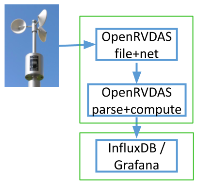
The logging machine runs all of OpenRVDAS: the front-line loggers (read, timestamp, write raw to disk, broadcast) and the loggers that parse and compute derived values. The second machine runs the database and Grafana. The parsing loggers reach it simply by pointing their database writer at the second machine’s address instead of localhost.

This guards against the two most common ways a busy installation hurts its own logging. A database that grows until it fills its disk fills the database machine’s disk, not the one the raw logfiles are being written to. And a heavy display load — a room full of scientists browsing dashboards, a runaway query, a Grafana upgrade gone wrong — competes for the second machine’s CPU and memory, not the loggers’.

Three machines: isolate the front-line loggers too. For truly robust operation, also separate the front-line loggers from everything downstream of them — parsing, derived data and the rest:

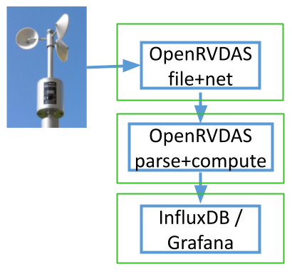
The first machine now does nothing but read the instruments, write the raw records to disk and broadcast them. A second runs the parsing and derived-data loggers, and a third the database and displays. A malformed record that crashes the parser, a derived-data logger that spins out of control, or a configuration change to the computations then can’t touch the machine holding the serial ports. That machine is so simple that there’s little left to go wrong with it.

The relay from the front-line machine to the parsing machine uses the same mechanisms the loggers already use, reaching across machines instead of across processes:

• UDP broadcast is the lightweight default: the front-line loggers’ UDPWriters already broadcast to the subnet, and the parsing machine’s parse_data logger just runs its UDPReader there instead. If a firewall sits between them, the data ports (6221–6226 by convention) must be open, per section 3.
• The cached data server is the alternative when you want delivery guarantees or to cross subnets: writers point their data_server at host:port rather than localhost, and CachedDataWriter buffers through interruptions.

In either arrangement, where the pieces land is pure configuration: the cruise definition’s variables name the UDP destination, data server and database URL, so moving a tier to another machine is a variables change, not a redesign. The shoreside replica above is the same idea stretched over a satellite link — and a second OpenRVDAS installation elsewhere on the ship can always subscribe to the first one’s CDS, which is how systems like CORIOLIX build on OpenRVDAS without touching its loggers.